DataSplash User Manual

Permission to use, copy, modify, and distribute this software and its documentation for any purpose, without fee, and without a written agreement is hereby granted, provided that the above copyright notice and this paragraph and the following two paragraphs appear in all copies.

IN NO EVENT SHALL THE UNIVERSITY OF CALIFORNIA BE LIABLE TO ANY PARTY FOR DIRECT, INDIRECT, SPECIAL, INCIDENTAL, OR CONSEQUENTIAL DAMAGES, INCLUDING LOST PROFITS, ARISING OUT OF THE USE OF THIS SOFTWARE AND ITS DOCUMENTATION, EVEN IF THE UNIVERSITY OF CALIFORNIA HAS BEEN ADVISED OF THE POSSIBILITY OF SUCH DAMAGE.

THE UNIVERSITY OF CALIFORNIA SPECIFICALLY DISCLAIMS ANY WARRANTIES, INCLUDING, BUT NOT LIMITED TO, THE IMPLIED WARRANTIES OF MERCHANTABILITY AND FITNESS FOR A PARTICULAR PURPOSE. THE SOFTWARE PROVIDED HEREUNDER IS ON AN "AS IS" BASIS, AND THE UNIVERSITY OF CALIFORNIA HAS NO OBLIGATIONS TO PROVIDE MAINTENANCE, SUPPORT, UPDATES, ENHANCEMENTS, OR MODIFICATIONS.

Introduction

This document is the user manual for the Tioga DataSplash (version 0.1) database visualization system developed at the University of California at Berkeley. Tioga DataSplash (formerly known as Tioga-2) allows users to interactively create and browse visualizations of database tables. DataSplash integrates two main components, a paint program and a navigation system.

As in a conventional paint program, the DataSplash user is presented with a palette of displayable objects (point, line, etc.). To draw an object, the user selects the corresponding paint primitive from the paint palette and places it in a two-dimensional canvas. A single such object is called a trim object. Examples of useful trim objects include titles and legends.

Unlike a standard paint program, DataSplash contains a window that shows rows from a database table to be visualized. Each row is assigned an x,y location in the canvas, i.e., the rows are scattered across the canvas, giving an effect similar to a scatter plot. For example, if the user has a table of United States cities with latitude and longitude columns, x and y can be assigned to the longitude and latitude values of each city.

At any point, the user can select an object in the canvas and duplicate it for every row in the database table. As a result, a copy of the object appears at the x,y location of every row in the table. The effect is like splashing paint across the canvas, coating every scattered row; these are splash objects. The user may also associate display properties of objects with columns in the table, e.g., height, width, color, and rotation of each splash object can be derived from values in the columns of its row.

DataSplash incorporates a sophisticated navigation model. Users can pan, zoom, teleport, and link to other canvases. Objects change representation as users zoom closer to them. DataSplash provides a unique mechanism, a layer manager, which allows end users to visually program the way objects behave during zooming. DataSplash also provides portals (formerly known as wormholes, portals are windows which go to other canvases). DataSplash users can automatically generate a portal for every row in a database table. Suppose the user has a canvas with a map of the United States. The user can easily specify that each city in the United States map should have a portal which goes to a map of that city.

The DataSplash developers are interested to learn how people use DataSplash; this is, after all, part of our research! If you develop a DataSplash visualization that you are willing to share with us, please send mail to datasplash@cs.berkeley.edu.

There are several other interesting visualization projects. The interested reader is referred to http://tioga.cs.berkeley.edu:8000/tioga/research.html#related_work for more information.

What is and is not in this document?

This manual contains usage information for the features of DataSplash, an overview of the system model, and a description of the sytem requirements.

This document does not provide a tutorial for using the system. However, there are tutorials included with the software. To access these, open datasplash/doc/tour_index.html on your local machine. Tutorials are also available at http://datasplash.cs.berkeley.edu/tour_index.html.

This user manual does not document any of the system source code for the program. Currently there is no plan to write a programming guide or to provide technical support for modifying the software source code.

Please direct all corrections, suggestions, and questions regarding this manual to: datasplash@cs.berkeley.edu.

Acknowledgements

The Tioga project is sponsored by NSF under grant IRI-9400773 and grant IRI-9411334 (UC Berkeley Digital Library Project).

We want to thank Brian Paul for the use of:

Mesa (Copyright © 1995-1996 Brian Paul)
The Mesa software can be obtained at: ftp://iris.ssec.wisc.edu/pub/Mesa.

We also want to give special thanks to T.C. Zhao and Mark Overmars for the use of:

XForms (Copyright © 1996 T.C. Zhao and Mark Overmars)
The XForms software can be obtained at: http://bragg.phys.uwm.edu/xforms.

Members of the Tioga project are faculty, staff, and students of the Database Research Group of the Computer Science Division, Dept. of EECS at the University of California at Berkeley. Faculty members of the group are Michael Stonebraker and Alex Aiken. Current students are Michael Chu, Chris Olston, Mybrid Spalding, and Allison Woodruff.

Former members of the Tioga project include Jolly Chen, Mark Lin, Nobuko Nathan, Caroline Paxson, Alan Su, and Jiang Wu. We would like to thank Mark Lin for a wonderful job on a first prototype of DataSplash.

We would like to thank Paul Aoki and Joe Hellerstein for valuable design input. We would also like to thank Paul Aoki for technical assistance.

System Requirements

The DataSplash binaries have been tested and compiled on the following platforms:

Operating System
Processor	Operating System
Dec Alpha	DEC OSF/1 3.2
HP	HPUX 9.0
Intel x86	Linux 2.0.24 ELF
Sun Sparc ®	Solaris 2.5.1

Binary versions for these platforms are available.

We are currently in the process of porting the software to other UNIX platforms.

The graphics package used in DataSplash does not require any special graphics card, nor will it take advantage of any. However, a Silicon Graphics source code port of the OpenGL-compatible parts of our implementation is underway to take advantage of the SGI graphics hardware.

In addition to the DataSplash requirements, you'll also need access to Postgres95 version 1.2 or later.

Postges95 can be downloaded from the DataSplash web site or from: http://www.postgresql.org.

System Overview

What is a DataSplash visualization and what can I do with it?

A DataSplash visualization is a graphical representation of database tables. You can browse a visualization by flying over a two-dimensional canvas in a three-dimensional coordinate system. You can also interactively modify the visualization. However, any changes you make to the representation of the data are not propagated to the original tables, i.e., DataSplash is not an update system for Postgres95.

How do I browse a DataSplash visualization?

You browse a visualization in the studio window. It's important to note that this is the same window you use to interactively edit the visualization. As a result, browsing and editing are very tightly integrated.

All navigation is performed with a one-button mouse (no function keys, control keys, or other keyboard actions are used for navigation). Mouse actions in DataSplash are interpreted according to your current mode. You choose this mode with the toolbar in the studio window.

In DataSplash, most objects are placed in a two-dimensional canvas. Imagine that you have a camera that is always above and pointed at the canvas. You can pan across the canvas. You can also zoom in or out above the canvas. The canvas is an infinite plane. The canvas exists at a particular elevation, called zero elevation. The camera cannot zoom beneath the canvas; however, there is no limitation on how high above the canvas a camera can zoom. A canvas consists of layers; as you zoom, different layers of the canvas become visible. In this way, you get different information as you zoom into the canvas.

In addition to panning and zooming, there are various ways to teleport to exact locations in the canvas. The most notable is the ability to teleport to the x,y coordinates of a particular table row.

Some canvases have special objects called portals, which are windows and links to other canvases. If canvas A has a portal onto canvas B, zooming through the portal positions you above canvas B. Specifically, if you position the camera above the portal in canvas A and zoom to zero elevation, you will go through the portal.

How do I create a DataSplash visualization?

Creating a DataSplash visualization does not require you to compile or write code. Instead, you use a paint program interface to draw and manipulate objects.

How do I create objects?

The main DataSplash window is called the studio. As mentioned above, you can browse or create visualizations in the studio. For the purpose of creating visualizations, the studio contains a simple paint program interface. You can create two types of objects, trim and splash.

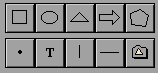
As in an conventional paint program, the studio contains a paint palette of displayable objects (point, line, rectangle, ellipse, triangle, polygon, arrow, and text). To draw an object, you select the corresponding primitive from the paint palette and place it in the studio canvas. A single such object is a trim object and is not data-dependent.

Unlike a standard paint program, DataSplash contains a window that shows rows from a table to be visualized. Each row is assigned an x,y location in the canvas, i.e., the rows are scattered across the canvas, giving an effect similar to a scatter plot. For example, if the user has a table of United States cities with latitude and longitude columns, x and y can be assigned to the longitude and latitude values of each city.

At any point, you can select an object in the canvas and duplicate it for every row in the database table. As a result, a copy of the object appears at the x,y location of every row in the table. The effect is like splashing paint across the canvas, coating every scattered row; these are splash objects. Note that you transform a trim object into a splash object by setting a property of the object. As a result, you can toggle any of the objects between trim and splash at any time.

You can also associate display properties of objects with columns in the table, e.g., height, width, color, and rotation of each instance of a splash object can be derived from values in the columns of its row. For example, one of the provided tutorials is a visualization of weather station data from four different states in the US. The table contains the latitude, longitude, and elevation of each station. Each row is located at the position of its longitude,latitude values. A triangle is drawn for each row and the height of each triangle is the elevation value in its row.

After you have created your objects, you are ready to program them for navigational interaction.

How do I program the behavior of objects during navigation?

DataSplash objects have three primary behaviors during navigation. You can program all three in the user interface.

First, you can use a dialog to program portals, i.e., you can link different canvases together. In addition to being links, portals are also windows that show the linked-to visualization.

Second, you can create sticky objects. While non-sticky (default) trim and splash objects are embedded in a two-dimensional canvas, sticky trim objects are painted on the lens of your camera. Therefore, as you pan and zoom they remain a constant size and stay in a constant position on the screen. These objects are particularly useful as titles, keys, legends, and other visual explanations and cues.

Finally, you can use the layer manager to program the behavior of objects during zooming. All objects in a canvas are organized into layers. Each object is in exactly one layer. As in traditional paint programs, these layers can be made invisible or visible individually. Unlike traditional paint programs, DataSplash allows you to control the elevation at which each layer is visible. You do this by graphically resizing layer bars in a layer manager (also known as an elevation map). Therefore, you can create visualizations which look different at different elevations (i.e., when the camera is at different distances from the canvas, the canvas looks different). For example, an object represented as a point at a higher elevation can be represented as text at lower elevations.

What kind of data can DataSplash visualize?

DataSplash currently visualizes the following three types of data:

types convertible to floating point
text strings
Postgres95 polygons.

The graphics package used in DataSplash recognizes only one floating point type (for portability reasons). Currently this type is a single-precision floating point number. All Postgres95 floating point and integer types recognized by DataSplash are converted internally into single-precision floating point.

The graphics library used to draw text can render only a single line of text. This one-line formatting doesn't display special characters such as tabs or new lines. Further, DataSplash internally limits the number of bytes of text input by the user to 1024 bytes. Any text input by the user (in a text box) which is longer than 1024 bytes is truncated or ignored. However, because DataSplash recognizes Postgres95 large objects, there is no limitation on the length of text fields in tables. Remember, however, that all text is displayed on a single line.

Any Postgres95 polygon can be rendered without modification, including polygons stored as large objects in the database.

DataSplash-recognized Postgres95 types
Postgres95 Type	Meaning
int	alias for int4
integer	alias for int4
int2	two-byte signed integer
int4	four-byte signed integer
float	alias for float4
float4	single-precision floating-point number
float8	double-precision floating-point number
smallint	alias for int2
text	variable length array of characters
polygon	two-dimensional polygon

When Postgres95 responds to a query from an application, it usually formats the data as a text string. Thus, any type of data in Postgres95 can be used by DataSplash if it is treated as a text string. If a Postgres95 data type is missing from the above table and you would like to see that type added to DataSplash (to be displayed as a text string), email your request to us. We will try to add these types over time.

What is the relationship between a visualization and the database?

The current DataSplash database interface is very simplistic. During visualization, DataSplash copies tables and their schema in their entirety from Postgres95 into main memory. This happens even if the visualization uses only part of a table. DataSplash does not currently take aggregates on tables, nor does it require any indexes. Once a table is read into memory, the system does not reference the database again. Therefore, no updates or modifications to a table appear unless you close the canvas and re-open it. We plan to provide a more sophisticated interface in the future.

Most transactions sent to the database on behalf of DataSplash are sent in one query. The only exceptions occur when the system needs to access a table with large objects and when a visualization is being saved or deleted from a database. However, no transaction spanning multiple queries to the Postgres95 database backend ever blocks on user input when sending the queries.

How are visualizations organized and stored?

Visualizations are composed hierarchically. Each visualization is called a canvas. A canvas contains an arbitrary number of layers. Each layer is associated with precisely one database table and each layer contains a number of visual objects. The properties of the visual objects (e.g., color, geometry, and spatial position) are determined by values from the database table associated with the layer.

DataSplash stores saved visualizations to a Postgres95 database. The components of DataSplash visualizations are stored in DataSplash-specific Postgres95 tables. DataSplash visualizations currently cannot be stored or read from arbitrary files on disk, although such flat files can be extracted from and imported to Postgres95 databases. See the Command Line Options section for further details on extracting and importing visualizations.

DataSplash visualizations are not stored in a binary format. Instead, they are stored in text form as a string of a context-free grammar. These files are easily read by humans or programs. Thus, other applications could be modified to export to or import from the DataSplash system. Please contact the Tioga reseach group if you would like further details.

What tables are used for storage by DataSplash?

DataSplash uses six tables for storing object name and object body by object type. In addition, any number of large object tables will be created for storing the object bodies as well.

Postgres95 tables used by DataSplash
Table Name	Use
comp_name	Canvas name table
comp_obj	Canvas object table pointed to by the canvas name table
ovly_name	Layer name table
ovly_obj	Layer object table pointed to by the layer name table
disp_name	Display object name table
disp_obj	Display object object table pointed to by the display object name table
Xinx######, Xinv######	Large object tables (a pair for each object) pointed to by any object table

Postgres95 has an internal limitation that any attribute of a table larger than 8K bytes in size be stored as a large object. If an object in DataSplash is less than 8K bytes in size, it is stored in its respective object table. Otherwise, a large object (table) is created for the object and the name for that large object is stored in the respective object table.

Warning! It is possible to manually delete items from the DataSplash tables without using DataSplash. This is not recommended. Please use the DataSplash purging mechanisms. These will safely delete any and all large object tables associated with DataSplash objects.

What does the installation include?

In addition to the DataSplash binary, the following document files, data sets, and DataSplash demonstration visualizations are included with the distribution. A list of tables used by the system internally is in the section What tables are used for storage by DataSplash?

Files
Contents	File
Program	datasplash/bin/datasplash
Installation Instructions	datasplash/INSTALL
GNU Library License Agreement	datasplash/LICENSE
Copyright Notice	datasplash/copyright_notice
User Manual	datasplash/doc/datasplash_user_manual.html
Index of Tours (Tutorials)	datasplash/doc/tour_index.html
Getting Started	datasplash/doc/tour_getting_started.html
Quick Tour	datasplash/doc/tour_quick.html
Splash Tour	datasplash/doc/tour_splash.html

Data Sets
Contents	Table Name
The top Fortune 100 companies by 1994/1995 rank	fortune100
US Census Bureau largest fifteen metropolitan regions (cities), broken down by age	top15_age
US Census Bureau largest fifteen metropolitan regions (cities): median income	top15_income
US Census Bureau largest fifteen metropolitan regions (cities): commute time	top15_time2work
US Census Bureau largest fifteen metropolitan regions (cities): transportation usage (public, car, walking, etc.)	top15_trans
Continental US polygons	state_polygons
Selected continental US polygons	state_polygons_reduced
Neveda, Utah, California, and Arizona polygons	nuca_polygons
Neveda, Utah, California, and Arizona weather station locations and elevations	nuca_station
Sample Cartesian coordinate system	grid
Sample Cartesian coordinate system	grid2

Visualizations
Contents	Name
US polygon visualization displaying the average commute time for the fifteen largest metropolitan regions (used in the Quick Tour)	us_timetowork
US average commute time bar chart for the fifteen largest metropolitan regions (used in the Quick Tour)	city_timetowork
Neva, Utah, California, and Arizona polygons and weather station data (used in the Splash Tour)	splash_demo
Average housing cost versus income for selected states	housing_income
Fortune 100 company rankings and profits	fortune100_Profit
Fortune 100 company rankings and growth	fortune100_Growth

General Notes on the User Interface

Here are a number of general observations you may find useful:

Almost all windows in DataSplash are modal, including dialog boxes. This means that you must dismiss a window or dialog before the other windows in the system recognize mouse or keyboard input. The main menu and studio windows are the only exceptions; if no other windows are present, you can move the mouse focus freely among the main menu and multiple studio windows.
DataSplash only requires single-clicking with a one-button mouse. However, there are short-cuts that use other mouse buttons or double-clicking.
Currently, there is no on-line help in the Help main menu selection.
There is on-line help in the form of tooltips. If you hold the mouse over most DataSplash buttons for a couple of seconds, a tooltip message should appear.

Document Conventions

DataSplash uses only the left (primary) mouse button, hereafter referred to as the "mouse button." The following definitions about the use of the mouse appear throughout this manual:

Click: press and release the mouse button quickly (single click).
Push: press and hold down the mouse button. A subsequent instruction will tell you when to release the mouse button.
Drag: move the mouse while holding down the mouse button. A subsequent instruction will tell you when to release the mouse button.

The following terminology is used to describe objects being rendered:

Solid: Objects are normally rendered as solid objects.
Wireframed: In certain situations, objects are rendered as a thin outline of their solid form (no fill is shown for these objects and their outline is shown at half width).

We provide links between different levels of this document to help you navigate. Specifically, the icon to the left of the heading of each subsection (e.g., , ) is a link to a higher-level section.

Main Menu

The main menu lets you create new visualizations or open and purge previously created visualizations. It also lets you configure several preferences for the system. These operations are enumerated on the File, Preferences, and Help menus.

File Menu

Open Database

All visualizations and tables are stored in the Postgres95 database management system. Postgres95 divides user space into areas called databases. When you select the Open Database command, you are asked to set the current database.

A DataSplash visualization is always stored in the database that was open when the visualization was first created. However, you may open visualizations from different databases during your DataSplash session (in fact, you may open them simultaneously in different studios). Further, different tables in the same visualization may be taken from different databases.

New Canvas

The New Canvas menu selection has a shortcut button on the main menu toolbar.

When you select this item, you are prompted with the Open Database dialog if you haven't opened a database yet. You are then prompted with the New Canvas dialog. The New Canvas dialog requires a canvas name before you can start a new visualization. (This is a little unusual, but there's a good reason for it. All layers are given a default name based on the canvas name. For example, if you name your canvas "foo," then the first layer within the canvas will be given the default name "foo_1.") You also need to choose whether to start with an existing layer or a new layer. By default, the New Layer button is enabled.

Once you've dismissed the New Canvas dialog, you asked for a couple of other pieces of information. Instructions appear in the Layer Manager sections: Create a New Layer or Add an Existing Layer.

The remainder of this section discusses default values that are assigned when you open a new canvas. Every canvas has a canvas start position. (When you first open the canvas, the camera starts at this position. Further, when you click the Home tool button on the toolbar and or the Go Home button in the Canvas Operations dialog, the camera teleports to this location.) Every canvas also has a maximum elevation for the layer manager (the tick marks in the layer manager represent percentages of this elevation). When a new canvas is created neither the canvas start position nor the maximum elevation has been set. The system tries to guess good default values by sampling a few records in the table associated with the first layer. The sampling algorithm looks at the x,y columns the user specified for the layer's table. The system determines some z elevation such that any and every splash object positioned at the sampled records' x,y position could be visible in the canvas camera for some x,y of the canvas. This z elevation is multiplied by two to become the layer manager maximum elevation and the x,y,z becomes the default starting camera position for the new canvas.

The default canvas start position and the default layer manager maximum elevation may be inappropriate for your application. It is always a good idea to set these two values yourself as soon as possible when you are creating a new visualization.

You probably don't want to assign the canvas start position a greater z value than the layer manager maximum elevation. In our experience, users find this confusing and inconvenient.

Open Canvas

The Open Canvas menu selection has a shortcut button on the main menu.

When you select this item, you are prompted for the name of an existing canvas to open. After you select a canvas, a new studio window displaying the canvas appears. The camera is positioned at the canvas' starting camera position.

Purge Components

When you select this item, the Purge window appears. This window allows you to remove existing canvases and layers from a database. The Purge window has two lists, one which shows a list of canvases and one which shows a list of layers associated with the currently selected canvas. There is a canvas selection in the Canvas list labeled "SHOW ALL LAYERS." This is not actually a canvas. It is simply a selection which will show all layers in the Layers list. When you have highlighted the items you wish to purge, click the OK button.

When you purge a canvas, the canvas is removed from the database, but all the layers it contains are left in the database (unless you explicitly purge these as well). Purging a layer is different from deleting a layer in the studio. When you delete a layer from a canvas in the studio, that layer no longer appears in that canvas. However, it remains in the database and may still be used in other canvases. When you purge a layer, on the other hand, it is actually removed from the database and cannot be used in other canvases.

A word of caution: don't let the Canvas and Layers lists in the Purge window mislead you. Layers in DataSplash can be shared among canvases. Purging a layer associated with one canvas will purge it for all canvases. Any canvas referring to a purged layer is no longer a legal canvas and is unusable by the system. You cannot open any canvas which refers to a purged layer. If you try, the system will respond with the following:

ERROR: Action Failed! Layer Not Found: <canvas name>.

Currently, the only way to determine if a layer is being used by some canvas is to traverse the Purge window Canvas list and check to make sure the layer is not used in any canvas.

Exit

When you select this item, the program exits (after presenting you with a confirmation dialog). The main menu window and all studio windows will close.

Preferences Menu

The Preferences menu lets you set several presentation options. These options apply to every studio window that is open.

Portal Depth

Portals may be arbitrarily nested. For example, imagine a portal in canvas A which shows canvas B. Canvas B may contain a portal onto canvas C. Indeed, if you have a portal in canvas A onto canvas A, you can have infinite nesting.

Portal depth controls whether portals are actually rendered. Portal in canvases lower than the portal depth are not rendered.

There are two reasons you may wish to control portal depth. First, rendering portals can be expensive. For example, if the tables for a portal canvas are relatively large, then that canvas may consume significant amounts of memory. Second, rendering portals at deeper levels of nesting is not always useful since they are often very small. For both of these reasons, the portal depth is set to one by default.

When the portal depth of a canvas is less-than or equal-to the current portal depth set in the Preferences menu, the portal canvas is rendered. This can happen when you change the portal depth preference or when you go through a portal. Once a portal canvas is opened, it is not closed until the studio containing the portal is closed (it is not closed even if the portal depth is set to a value at which it is not rendered).

Portal Effects

This command gives you control over the quality of the animation effects occurring when you go through a portal. Changing this value is an optimization feature. Slower effects take longer to render, but have more detail. Faster effects render more quickly, but have less detail.

Zooming Style

Zooming style determines the behavior of Interactive Zoom mode. There are two styles, logarithmic and linear.

By default, interactive logarithmic zooming is enabled. Logarithmic zooming increases/decreases your distance to/from the canvas by a factor 1/2 of the starting elevation when you drag the mouse the entire length of the canvas. For example, if you are zooming into the canvas starting at elevation 100 and you drag the mouse once across the entire distance of the canvas, you decrease your elevation from the canvas by 50%, i.e., you end up at elevation 50. If you drag the mouse again across the entire distance of the canvas, you again decrease your elevation by 50%, which means you end up at elevation 25.

Note that in theory you could never get to zero elevation using logarithmic zooming, which implies you could never go through a portal. For this reason, logarithmic zooming has been slightly modified so that you can enter a portal using logarithmic zooming (a small constant is added to the zooming distance).

The other zooming style is linear. You can set the zooming style to use a constant linear speed during interactive zooming. The constant speed is not user-configurable; it is based on the layer manager maximum elevation. This zooming style is useful when you wish to use the layer bars to control the amount of time a layer is visible. For example, any layer bar which is twice as long as some other layer bar in the layer manager takes twice as long to zoom past when using linear speed zooming in the canvas.

Static Rendering

Objects can be rendered in two ways, solid or wireframed. Wireframed objects are only rendered as a thin outline of the normal objects (no fill is shown for these objects and their outline is shown at half width). Wireframed objects render significantly faster than solid objects.

Static rendering occurs when the mouse is not being dragged in the canvas, i.e.,you are not panning or zooming interactively.

If you feel your rendering performance is slow due to the graphics software, try setting the Static Rendering option to wireframe.

Interactive Rendering

See Static Rendering for an explanation about wireframe rendering. Interactive rendering occurs when the mouse is being dragged in the canvas. By default, the Interactive Rendering wireframe option is enabled to enhance performance during panning and zooming.

Show 3-D Box

You can choose to show a three-dimensional box while you are panning and zooming. Some people find the box helps to orient them.

Help Menu

There is currently no on-line help.

About Tioga DataSplash

When you select this item, a screen with information about the system appears.

Show Tooltips

You can turn tooltips off and on with this item.

Studio

Several DataSplash components are used to edit or navigate in a visualization. These components are grouped together in a window called a studio. A new studio is created each time you open a canvas using File menu Open Canvas.

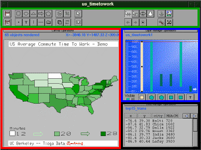
Figure 1: The studio.

Studio Layout

The studio is broken into four distinct areas as highlighted in Figure 1.

Toolbar Area (boxed in green)

The toolbar buttons occupy two rows at the top of the studio. Most of the tools in the toolbar represent the current mode of the studio (e.g., you can be in pan mode). The mode defines the way that mouse actions in the canvas and layer manager are interpreted. There are modes for creating and editing objects and for navigating.

Canvas Area (boxed in red)

The canvas is the large square area on the lower-left side of the studio. The canvas displays the current visualization. You can pan and zoom in the canvas, as well as create and edit objects in the canvas. The Canvas Area also contains a message window. Above the message window is a long button bar.

Layer Manager Area (boxed in blue)

The layer manager occupies a sky blue area in the upper right of the studio. The layer manager is used to graphically program different layers in the canvas. The layer manager also displays the current elevation of the camera. Like the Canvas Area, the Layer Manager Area contains a message window and a long button bar.

Data Manager Area (boxed in black)

The data manager occupies a gray area in the lower-right of the studio. The data manager displays the current database table. Like the other two areas, the Data Manager Area contains a message window and a long button bar.

Toolbar Area

The toolbar contains the tools used to edit and browse a visualization. The toolbar spans the top of the studio. Most of the tools in the toolbar represent the current mode. The studio is always in exactly one mode. A mode defines the meaning of mouse movements in the canvas and layer manager. For example, when a studio first appears, it is in Click Pan mode.

To select a mode, simply click on the corresponding button in the toolbar. The button representing the current mode is depressed.

Only four of the modes described below - Save, Save As, Select, and Erase - apply to both the canvas and the layer manager. The other modes apply to the canvas only. When you are in a mode that applies only to the canvas, the layer manager is in Select mode.

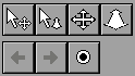
Only four of the tools described below are not modes: Home, Portal Back, Portal Forward, and Close. These tools are actions and do not change the current mode of the studio.

Save Group

The group of tools in the upper-leftmost corner of the studio (see Figure 1) is the Save Group. When you are in one of these modes, the mouse cursor changes to an "X" when positioned over the canvas (clicking the mouse in the canvas does nothing). The mouse cursor changes into a floppy disk when positioned over a layer bar in the layer manager.

Save

DataSplash allows layers to be shared among canvases, which means that modifying and saving a layer in one canvas may affect another canvas. As a result, DataSplash allows you to save three different types of objects: when you enter Save mode, you can save the entire canvas (including the layer manager program and every individual layer), the layer manager program only (the names of layer bars in the layer manager as well as their ordering and top-and-bottom positions, as described in the part of this manual which discusses the layer manager), or individual layers. Currently, there is no way to individually save or reuse specific objects within a layer.

In Save mode, all unsaved components are visually highlighted by a bright pink color. Clicking the mouse on one of these pink-colored components saves it. Items that have not been modified since they have been saved are a burgundy color. When you save an item, it changes from pink to burgundy.

To save the entire canvas, enter Save mode and click on the button bar positioned immediately above the canvas in the studio (this button spans the entire width of the canvas and is labelled Save Everything in Save mode). This is the equivalent of using Save in the File menu in most other applications.

You may save the layer manager program independently (i.e., without saving changes to the layers themselves). To save the layer manager program only, enter Save mode and click the button bar positioned immediately above the layer manager in the studio (this button is labelled Save Layer Manager in Save mode).

Finally, to save an individual layer, click on its layer bar in the layer manager.

DataSplash supports write-protection of layers and canvases. Modified and protected layers are colored fuchsia in Save mode. In Save mode, if you try to save a layer or canvas that is write-protected, you get a Warning dialog. You can easily override the write protection by clicking the OK button in the Warning dialog. (To learn how to make a layer or canvas write-protected, see Save As mode.)

Save As

Save As mode is similar to Save mode; please refer to the discussion presented there. The primary difference in Save As mode is that it allows you to rename objects when you save them. Also, in Save As mode, you can make a layer or canvas write-protected.

In Save As mode, saving the canvas under a different name has no effect on the layers. They retain their original names. If you wish to rename all the layers within a canvas, you must do so by renaming each individual layer in Save As mode. There is a shortcut to rename all layers within a canvas based on the name of the canvas. In Save As mode, the long button bar immediately above the layer manager is the Rename and Save All Layers button.

Saving either a canvas or a layer under a different name does not purge the original from the database.

Paint Palette Group

The second group of tools from the left in the toolbar (see Figure 1) is the Paint Palette group. This group contains drawing primitive modes. When you are in one of these modes, the mouse cursor changes to a pencil when positioned over the canvas. When you push, drag, and release the mouse, the object specified by the tool appears.

Specifically, with the exception of Polygon objects, all Paint Palette objects are drawn by specifying two corners of an object's bounding box. The first point is the point on the canvas at which you push the mouse. The second point is the point at which you release the mouse (after dragging it to the desired location). An outline of the object's bounding box is shown as you draw the object. After you release the mouse, DataSplash automatically switches to Select mode and selects the object you just drew.

All objects are drawn in the selected layer. If you try to paint an object in the canvas when the selected layer is not visible, an Error dialog appears. See the Layer Manager section for further details.

To edit the object after you draw it, use tools in the Rotate or Select groups.

If rendering performace is slow when you pan and zoom, be patient when painting objects in the canvas. When you push and drag the mouse in the canvas, the canvas is rendered continuously to show the bounding box as it changes. To improve performace, either turn off all layers except your drawing layer, or pan to a relatively empty area of the visualization.

Rectangle

The sides of the rectangle are equivalent to the sides of the bounding box. Rectangles are the basis for portals. See the Format Dialog section for more details.

Point

The bounding box size does not determine the size of the point; the point is simply centered in the bounding box. Use the Line Width pop-up menu in the Format dialog to change the point size (which is represented in pixels). A point is rendered as its point size regardless of elevation.

Draw a large bounding box to make the point easier to select at higher elevations.

Oval

The sides of the bounding box drawn for the oval determine the size of its major and minor axes.

Text

Unlike the bounding boxes for all other objects, the bounding box for text does not bound the entire text object . Instead, the bounding box for a Text object is associated only with the first letter of the text.

In addition, the system defaults to the word "Text" whenever you draw a Text object. You use the Text Specific button in the Format dialog to change the word "Text" to something more appropriate or to associate the Text object with text taken from a table.

Note that text line width is rendered as its point size (in pixels) regardless of elevation.

Triangle

The width of the bounding box determines the base of the triangle and the height of the bounding box determines the height of the triangle. This tool creates isoceles triangles only. You may use the Polygon tool to draw a non-isoceles triangle.

Vertical Line

The height of the bounding box determines the vertical length of the line. The width of the bounding box does not determine width or any other property of the line (although it is helpful to draw a large bounding box so that the object is easier to select). The vertical line appears at the middle of the width of the bounding box. Use the Line Width pop-up menu in the Format dialog to change the width of the line (the width of the line is represented in pixels). A line's width is rendered as its point size regardless of elevation.

You may use the Polygon tool to draw an arbitrary two-point line.

Occasionally, you may think you are in Horizontal Line mode when you are actually in Vertical Line mode. This has the apparent effect of creating a long invisible horizontal line, when in fact a very short vertical line is created.

Arrow

The height of the bounding box determines the height of the arrow and the width of the bounding box determines the arrow length. You can not modify the relative size of the head and line.

Horizontal Line

This is the same as Vertical Line mode except the width of the bounding box reverses roles with the height.

Polygon (Polyline)

You do not draw a bounding box to specify a polygon. Instead, you click the mouse in the canvas; every mouse click registers a new point for the polygon/polyline.

Once you have clicked the mouse to create a point, you cannot undo it. To erase a polygon/polyline that is in progress, click any other mode button on the toolbar. The partial polygon/polyline will be erased.

Polygon mode can be used to draw both polygons and polylines. You distinguish these when you finish entering the object. Specifically, when you are entering points for either a polygon or a polyline, there are two select handles, one at the first point entered and one at the last point entered. If you click the mouse on either handle, you finish entering the object. If you click on the first point entered, you create a closed polygon. If you click on the last point entered, you create a polyline. Polylines cannot be filled.

When you finish entering a polygon or polyline, the system creates a bounding box for the object, switches to Select mode, and automatically selects the object. After you have created a polygon or polyline, you can manipulate it using tools from the Rotate and Select groups.

A polygon drawn with the Polygon tool cannot use polygon data from a Postgres95 table. To create such an object, see User-defined Objects.

User-defined Objects

As with other objects, you create a user-defined object by drawing a bounding box. Once you have drawn the bounding box, a series of dialog boxes gathers information needed to complete the object.

For example, Postgres95 polygons are implemented as user-defined objects. If you wish to use Postgres95 polygon data, draw a bounding box for a user-defined object and choose either "tuple polygons" or "tuple polyline" from the Open Display Function dialog that appears. After you select one of these, you are asked to pick the column in the table that holds the polygon points. The shape of each polygon appears at the x,y location of the row containing that polygon. Note that the vertices of the polygon are corrected so that the polygon is centered at that x,y location.

One special consideration for Postgres95 polygons is setting the x,y columns of the layer so that the polygons are positioned correctly. To facilitate this, DataSplash allows the polygon column containing the points of the polygon to be used in the x,y columns specifying the location of each row. In this case, the x,y canvas position for a row is assigned automatically to the absolute center of the bounding box of the polygon contained in that row.

If you are interested in developing other display functions for DataSplash, please contact the Tioga research group.

Rotate Group

The third group of tools from the left in the toolbar (see Figure 1) is the Rotate group. This group contains modes in which you can manipulate objects you have created. When you are in one of these modes, the mouse cursor changes to the icon of the tool when positioned over the canvas. You can only manipulate objects in the selected layer. Before you manipulate an object, you must enter one of modes in the Rotate group and then select the object while in that mode (by clicking on it or rubberbanding it).

If you select multiple objects and use these tools, only a single, arbitrarily-chosen one of these objects is modified (unless, of course, you modify an instance of a splash object, in which case the changes to that object are automatically propagated to all the related splash objects).

Rotate

To rotate an object, click on or rubberband the object. Then push the mouse on one of the handles of the object and drag the mouse. Release the mouse when the object is in the desired position (the object will rotate around its center). The system does not allow you to rotate any splash object which is not center-aligned. When you try to rotate such an object, nothing happens (you do not receive an Error dialog).

Duplicate

When you select an object in this mode, the object is duplicated and the copy appears in the center of the canvas. All duplicating occurs in the selected layer. There is no cut-and-paste mechanism.

Flip Vertical

When you select an object with this tool, it flips vertically.

Flip Horizontal

When you select an object with this tool, it flips horizontally.

Select Group

The fourth group of tools from the left in the toolbar (see Figure 1) is the Select group. This group consists of two modes: Select and Erase. When you are in one of these modes, the mouse cursor changes to the icon of the tool when positioned over the canvas. Select and Erase modes apply to both the layer manager and the canvas.

Note that selecting a splash object has a special meaning in DataSplash. When you modify an instance of a splash object, that change automatically propagates to the other instances of the splash object.

Note that only three operations (Erase, Move, and Resize) are defined for groups of selected objects. If you perform other operations on a group of objects, they either have no effect or affect an arbitrary single object (if the object is a splash object, the changes propagate).

Select

You can select an object in two ways. First, you can click on an object in the canvas (or a layer bar in the layer manager). This is called click-select. Second, you can push the mouse and drag it to rubberband part of the canvas (this technique does not apply in the layer manager). As you are dragging the mouse, a box outline appears to show the rubberbanded area. When it is the desired size, release the mouse. This method is called rubberband select and it is especially useful for selecting multiple objects.

When an object is selected, multiple bounding box points appear for the object. When you position the cursor over any bounding box point on the border, it turns into crosshairs. If you press the mouse button and move the cursor while keeping the button pressed, the object changes size (it resizes proportionally if you select a corner point). This is the Resize operation.

If you position the cursor over the bounding box point in the center of the object, the cursor turns into a hand. If you push the mouse button and drag the mouse, the object moves. This is the Move operation.

Finally, if you position the cursor within the bounding box but not on a bounding box point, the cursor becomes a microscope. If you click the mouse button at this point, the Format dialog box appears. You can use this dialog to edit properties of the object. See the Format Dialog section for more details.

Erase

Delete objects using the same gestures as in Select mode. See the important discussion in Select Group.

An erased object is not recoverable. There is no undo of any sort.

Erasing a layer bar in the layer manager removes the layer from the canvas, but it does not remove it from the database. Therefore, if you erase a bar, you can add it back in (see the section describing how to Add an Existing Layer).

Navigate Group

The fifth group of tools from the left in the toolbar (see Figure 1) is the Navigate group. This group contains tools for browsing visualizations. Observe that two of the tools, Portal Forward and Portal Back, are actions and not modes. When in one of the Navigate modes, the mouse cursor changes to the icon of the tool when positioned over the canvas.

Click Pan

The Click Pan tool changes the x,y camera position. When you are in Click Pan mode, the camera pans so that any location you click is centered in the canvas.

Portal Back

DataSplash maintains a list of all visited portal canvases. (This is very similar to the list of links visited in a web browser.) Pressing the Portal Back tool takes you to the previous canvas in the list. The icon is grayed-out if the back list is empty.

There are special effects that happen when you go back through a portal. You can use Portal Effects in the Preferences menu to turn them off or to change the speed of the effects.

Rubberband Zoom

The Rubberband Zoom tool allows you to automatically adjust your camera elevation and x,y position in the canvas. To use the tool, push and drag the mouse in the canvas to rubberband the area you wish to view. When you release the mouse button, the selected area fills the canvas.

The rubberband has the aspect ratio of the canvas.

Portal Forward

DataSplash maintains a list of all the portal canvases you have visited. (This is very similar to the list of links visited in a web browser.) Pressing the Portal Forward tool takes you to the next canvas in the list. The icon is grayed-out if the forward list is empty.

There are special effects that happen when you enter a portal. You can use Portal Effects in the Preferences menu to turn them off or to change the speed of the effects.

Interactive Pan

The Interactive Pan tool changes your x,y camera position in the canvas. When you are in Interactive Pan mode, the system updates the canvas continuously to follow any mouse drag. While you are dragging the mouse, the system renders the canvas objects as wireframed objects to improve performance. You can change this behavior by setting the Interactive Rendering preference in the Preferences menu.

Portal Click

Portal Click mode is shorthand for zooming to zero elevation and going into a portal canvas. This mode immediately links to a portal canvas similar to clicking on a hyper-link in a web browser.

Note that the system does not allow you to zoom into a portal contained in a layer bar that does not extend to zero elevation. It is possible, however, to enter such a portal using Portal Click mode.

There are special effects when you enter a portal. You can use Portal Effects in the Prefereneces menu to turn them off or change the speed of the effects.

Interactive Zoom

The Interactive Zoom tool changes the z camera canvas position, or elevation above the canvas. When you are in Interactive Zoom mode, dragging the mouse up or down in the canvas updates the canvas elevation continuously to follow the mouse drag. While you are dragging the mouse, the system renders the canvas objects as wireframed objects to improve performance. You can change this behavior by setting the Interactive Rendering preference in the Preferences menu. You can also change the zoom speed (logarithmic or linear) by setting the Zooming Style in the Preferences menu.

Studio Operations Group

The sixth group of tools from the left in the toolbar (see Figure 1) is the Studio Operations group. This group consists of four tools: Layer Translate, Layer Scale, Home, and Close. Two of these tools (Home and Close) are actions and not modes. When you are in one of the modes (Layer Translate and Layer Scale), the mouse cursor changes to the icon of the tool when positioned over the canvas.

Layer Translate

In Layer Translate mode, you can graphically program the functions that determine the x,y position of each row. The general procedure begins by selecting one object; an anchor appears over the selected object. When you move the anchor to a new location, the functions that determine the x,y position of each row are updated to incorporate this change. Specifically, layer translate changes the x,y constant term of the linear functions used to determine the x,y position of each row. (If you wish to change the multiplier, use Layer Scale mode.)

You can use Layer Translate to co-register two different layers that have the same x,y scale but are slightly offset. Observe that you can use the Layer Operations dialog to make the same change in a non-graphical manner.

To use this tool, perform the following operations (remain in Layer Translate mode throughout the entire sequence):

Enter Layer Translate mode.
Click or rubberband the object you wish to use as an anchor (use the same method as in Select mode). An anchor should appear over the object.
Move the mouse over the center of the anchor. The mouse cursor should turn into a hand.
Push, drag, and release the mouse. The anchor should move and the entire canvas should shift accordingly.

Layer Scale

In Layer Scale mode, you can graphically program the functions that determine the x,y position of each row. The general procedure begins by selecting two objects; anchors appear on each object. When you move either anchor to a new location, the functions that determine the x,y position of each row are updated to incorporate this change. Specifically, layer scale changes the x,y multiplier term of the linear functions used to determine the x,y position of each row. (If you wish to change the constant, use Layer Translate mode.)

You can use Layer Scale to co-register two different layers that have different x,y scales. Observe that you can use the Layer Operations dialog to make the same change in a non-graphical manner.

To use this mode, perform the following operations (remain in Layer Scale mode throughout the entire sequence):

Enter Layer Scale mode.
Click or rubberband the first object you wish to use as an anchor (use the same method as in Select mode). An anchor should appear over the object.
Click or rubberband the second object you wish to use as an anchor. An anchor should appear over the object.
Move the mouse over the center of either of the anchors. The mouse cursor should turn into a hand.
Push, drag, and release the mouse. The anchor should move and the entire canvas should be scaled proportionately.

Home

When you click the Home button, the canvas camera teleports to the canvas start (or home) position.

Close

When you click the Close button, the studio window closes.

Canvas Area

The canvas area contains the display of the current visualization. It is in the lower-lefthand corner of the studio and has three components: the canvas itself, the Canvas Operations button and the Canvas Message area. Both the Canvas Operations button and the Canvas Message area are immediately above the canvas in the studio.

Canvas

The canvas itself displays the current visualization. The name of the canvas is displayed as the title of the studio window. When the mouse cursor is positioned over the canvas, its shape is dependent on the current mode determined by the toolbar. You can navigate in the canvas, or create and edit objects. Editing objects is discussed in the Format Dialog section.

Canvas Operations Button

The long button at the top of the canvas area is the Canvas Operations button. When you click on this button in any mode other than Save and Save As, it invokes the Canvas Operations dialog.

When you are in Save mode, the label of the Canvas Operations changes to "Save Everything." See Save mode for details of the semantics of this button in Save mode.

When you are in Save As mode, the label of the Canvas Operations button changes to "Save Canvas." See Save As mode for details of the semantics of this button in Save As mode.

Canvas Operations Dialog

Canvas Background Color

You can set the color of the background of the canvas using the color sliders. The text box above each slider shows its current value. You can type directly into these text boxes. The current color is displayed in the box on the righthand side of the Canvas Operations dialog. Clicking the Default button restores the background to the system default color (light gray).

Canvas Teleport with Coordinate Display

The three text boxes in the middle section of the dialog box display and control your current x,y,z camera location. When the dialog first appears, these boxes reflect your camera location when you invoked the dialog. If you enter values into these boxes, the camera teleports to the corresponding location when you click the OK button in the dialog.

Canvas Protected

The Canvas Protected button is related to saving. Details appear in the discussion of Save mode. Enable this if you want a Warning dialog to appear before any changes to the canvas can be saved.

Move Home

When you click the Move Home button, the canvas start position is changed to the current values in the x,y,z coordinate display next to the Move Home button in the dialog.

Go Home

When you click the Go Home button, the camera teleports to the current canvas start position. The effect is identical to that of clicking the Home tool on the toolbar.

Max Elevation

The Max Elevation text box displays the current layer manager maximum elevation represented by the 100% tick mark in the layer manager. You may update this value.

Canvas Message Area

The Canvas Message area appears immediately above the canvas and below the Canvas Operations button. All messages are displayed in blue text. The lefthand side of the Canvas Message area provides useful status information and hints. The righthand side of the canvas message area displays your current x,y,z canvas camera location.

Format Dialog

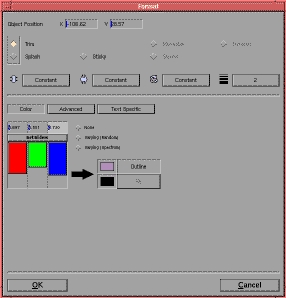
With the widgets in the Format dialog (see Figure 2), you can specify the type (trim or splash), color, rotation, bounding box height, bounding box width, point size, portal type and columns, text string values, alignment, and position of an object. To invoke the format dialog, select the object of interest and then position the mouse cursor over it until the microscope mouse cursor appears. Then click the mouse (see Select Group and Select).

A horizontal line divides the Format dialog. Below the line is a row of option buttons. When you click one of the option buttons, the related widgets appear in the space below.

Figure 2: The Format dialog.

Column-Based Values

A number of properties in the format dialog may be associated with values from columns in the database. In general, these properties are set using pop-up menus. Each pop-up menu contains a list of columns in the table of the selected layer, as well as the options "Function" and "Constant." When using one of these pop-up menus, bear in mind the following:

All the columns in the table associated with the selected layer are listed in the menus. Any column from the table which is not a DataSplash-recognized Postgres95 data type or which does not apply to the current object is grayed-out.
The "Function" selection contains a linear function. Choosing this option invokes a dialog. You can use this function to scale the column values. Note that when you choose a column from the pop-up menu list, the system picks some linear function that scales the data values. This linear function is based on a small sample of the table data. You may wish to edit it using the function dialog.
The "Constant" selection is identical to the "Constant" term of the linear function used in the "Function" selection.
When you are editing a trim object and you select a column from the pop-up menu list, the system changes the object into a splash object.

Object Position

The Object Position (X and Y) text boxes are in the top, upper-left corner of the Format dialog (see Figure 2). These boxes display current values; these can be updated. Their meaning is dependent on object type as follows:

Splash: The text boxes indicate each object's offset from the x,y position of the row.
You can also set these values graphically by using the mouse to drag a splash object in the canvas. If you want each splash object to appear at the precise x,y location of its row, set these values to zero.
Trim, but not Sticky: These values represent the precise x,y position of the trim object in the canvas. You can also set these values graphically by using the mouse to drag the trim object in the canvas.
Trim and Sticky: These values are meaningless. Ignore them.

Object Type

Object type is determined by the Trim, Splash, Portal, and Sticky buttons in the upper-left of the Format dialog (see Figure 2). The Splash and Trim buttons have a frame around them because only one can be enabled at a time. In other words, objects can either be data-dependent (splash) or not (trim). In addition, trim objects can either be sticky (painted on the camera lens) or not (embedded in the canvas). Finally, the Portal button only appears for rectangles; otherwise it is not shown.

Trim
When you first draw an object, it is a trim object by default. Trim objects do not have data-dependent position or properties and appear only once in the canvas.

Splash
If the object is of the splash type, one instance of the splash object is created for every row in a database table. The position of each instance of the splash object is determined by the x,y position of its row. Other properties of the object can be data-dependent as well, e.g., size or color.

Portal
Only rectangles can be of Portal type. A rectangle of type Portal is a visual link to another DataSplash visualization. Information about certain portal display properties appears in the section on Portal Type.

Warning! Enabling this button without setting the other portal properties in the Format dialog may result in strange behavior. See the Portal Specific button to learn how to set the other portal properties.

Sticky
Any trim object can be made sticky. A sticky, trim object is considered to be "painted on the lens" of the canvas camera and therefore does not move during panning or zooming.

Splash Wizard

When the Splash button in the Format dialog is enabled, the Splash Wizard series of dialog boxes appears. The Splash Wizard presents the opportunity to set the x,y columns for the selected layer. It also presents the opportunity to set the bounding box height, width, and rotation.

Portal Type

The Portal Type buttons are located right next to the Object Type buttons in the upper-right of the Format dialog (shown in Figure 2). Portal type only applies to rectangles which are of object type Portal; the Portal Type buttons are grayed-out for all other objects. In addition, the Slaved button is grayed-out for all portals except those that are sticky and trim. None of the Portal Type buttons are enabled by default.

A canvas containing a portal is called a parent canvas. Every portal goes to a canvas which we refer to as the child canvas. Every portal is linked to a specific x,y,z coordinate in its child canvas. The view through the portal is of the child canvas at that x,y,z location. When you go through the portal, the canvas camera goes to this location. The x,y,z values combined with portal type determine the way the portal is displayed when viewed in the context of the parent canvas.

Moveable
When this Portal Type button is enabled, moving the portal in the parent canvas updates the portal x,y values. The x,y distance moved in the canvas is added to the portal x,y values. The distance is calculated in terms of coordinates, not the number of pixels the mouse moved. Therefore, when you move portals at higher elevations above the child canvas, they change distance more quickly than when you move portals at lower elevations above the child canvas.

Dynamic
When this Portal Type button is enabled, a line-of-sight effect is created. Imagine you are standing to the left of a window and looking through it. Now imagine you walk to the right side of the same window. You will see two different views. This is a line-of-sight effect. More precisely, the portal is drawn using a true three-dimensional perspective: you are looking through a hole in the parent canvas onto the child canvas below in three-space.

Slaved
When this Portal Type button is enabled, the portal x,y,z coordinate is slaved to the studio canvas camera x,y,z. That is to say, the portal canvas x,y,z is some function of the parent canvas camera position. Specifically, you can create a constant offset between the two cameras using the Portal Specific options. This feature is only available for sticky, trim portals.

Bounding Box Properties: Height, Width, and Rotation

The bounding box property buttons are located in a row slightly above middle of the Format dialog (shown in Figure 2). There are three properties: height, width, and rotation. You can set each of these properties using a column-based pop-up menu next to its icon. Note that rotation units are in degrees, and the system rotates objects counter-clockwise. The height and width units are canvas units.

Line Width

The Line Width pop-up menu is located in the same row as the bounding box properties and has an icon of a number of lines of different widths. The pop-up menu sets the width of a line (or the size of a dot) to a specified number of pixels.

Color Button

The Color button is the first option button from the left (in the row in the middle of the Format dialog). It is always available. You can use the color portion of the format dialog to specify the outline and fill of an object by toggling between the Outline and Fill buttons. There are four possible types of color settings:

You can enter constant RGB values by clicking in the colored sliders or by typing values into the input boxes above the sliders (to update the colored sliders based on your input, press the "Set Sliders" button).
You can set the outline or fill to have no color by enabling the None button.
You can set the outline or fill of splash objects to be randomly colored by enabling the Random button. If you enable this button for a trim object, the object type automatically changes to splash. The heuristic that sets the colors of the objects tries to maximize visual contrast among objects that are located close together. Therefore, objects at the same x,y location have the same color, but objects with slightly different x,y values have contrasting colors.
You can base colors on a column in the current table by enabling the Varying Spectrum button. If you enable this button for a trim object, the object type automatically changes to splash. Use the pop-up menu to choose the column. Use the two values below the column name to choose the minimum and maximum values. Each of these values has an associated color. You can edit this color by clicking on the button by the arrow underneath the input box and then adjusting the RGB color bars.

Note that none of these changes take effect until you have clicked OK in the Format dialog.

Alignment Button

The Alignment button is the second option button from the left (in the middle of the Format dialog). It is always available. However, the widgets for this option are grayed-out unless the object is a splash object.

By default, each splash object is centered on the x,y position of the database row with which it is associated. You can click on one of the alignment buttons to change the alignment point for a splash triangle so it has a different relationship to the x,y position of its row. Note that you cannot rotate objects except when they are center-aligned.

Text Specific Button

The Text Specific button is the third option button from the left. It is only visible for Text objects.

Constant text may be applied to both trim and splash objects. To change this text, you must enable the button next to the text-input box. Then you can modify the Constant text box to arbitrary text consisting of fewer than 1024 characters (recall that it contains the default word "Text" when you first draw a Text object).

Attribute (column) text may be applied to splash objects only. To assign attribute text, first enable the button next to the dialog. Then choose a column from the pop-up menu.

Portal Specific

The Portal Specific button is the third option button from the left (in the middle row of the Format dialog). It is only visible for portals.

Every portal goes to a child canvas. The browser list on the left displays the list of canvases in the current database. Click on one of these to select the portal canvas. It is legal to have a child canvas be the same as the current canvas in the studio (i.e., the parent canvas).

On the right side of the Format dialog are pop-up menus used to set the portal x,y,z values. These values specify the spatial relationship between the parent canvas and the child canvas. Specifically, the x,y location in the child canvas is aligned with the center of the portal in the parent canvas. The z value is the distance between the child canvas and the parent canvas. This implies that the child canvas is viewed from the sum of the distance from the camera to the parent canvas and the distance between the parent canvas and the child canvas. For example, if the studio canvas camera is at an elevation of 50 z units over the canvas and is also over a portal, and the portal z coordinate has a z value of 10, the image displayed in the portal will be seen from an elevation of 50 + 10 = 60 z units.

The pop-up menus contain entries of the types detailed in the section on column-based values. The Default button immediately below the X,Y,Z pop-up menus sets the portal x,y,z values to be the canvas start (home) position of the child canvas.

Below the Default button are the Slaved Portal Type constant offset text boxes. These assign a constant offset between the slaved portal location and the current camera location in the parent canvas. These boxes are grayed-out except when the Slaved button is enabled.

Layer Manager Area

The layer manager controls the properties of all layers. Perhaps the most important of these is the elevation range at which each layer is visible.

The layer manager area has three components, the layer manager itself, the Layer Manager Operations button and the Layer Manager Message area. Both the Layer Manager Operations button and the Layer Manager Message area are immediately above the layer manager in the studio. Figure 3 shows these components.

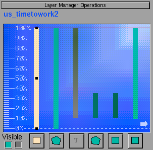
Figure 3: The layer manager area.

Layer Manager

The layer manager is the sky blue area in the middle of the right side of the studio (see Figure 3). Each vertical bar in the layer manager represents a single layer. The top of the layer bar represents the highest elevation at which the layer is visible. Similarly, the bottom of the layer bar represents the lowest elevation at which the layer is visible. The 100% tick mark and dashed line represent the layer manager maximum elevation set in the Canvas Operations dialog. The 0% tick mark and dashed line represent zero elevation.

Your current elevation is displayed by the thin cyan or red horizontal line. You can move the elevation bar by clicking on a tick mark on the left side. (This also works if you click anywhere in the layer manager except on a layer bar.) You can also drag the elevation bar to an elevation percentage of your choice. Note that the canvas does not update until you release the mouse. If you want the continuous zooming effect, use the Interactive Zoom tool.

In addition to vertical size and position, the ordering of the bars from left to right is also significant. In general, objects in a given layer are drawn on top of objects in layers to their left (i.e., layers are rendered from left to right). More precisely, all splash and trim objects are rendered from left to right. Then, all sticky objects are rendered from left to right.

If you create a portal, it is best to place it as late in the drawing order (i.e., in a layer as far to the right) as possible. Putting a portal in the rightmost layer guarantees that nothing is drawn over the portal.

Precisely one layer bar is selected at all times. Except when the studio is in Erase, Save, or Save As mode, you can Select a layer bar by clicking on it (it will turn the beige selected color). Just as you can move, resize, or edit the selected objects in the canvas, you can move, resize, or edit the selected layer bar. In this way, you can change the elevation at which a layer is displayed by using resize, you can change the drawing order by moving a layer, or you can change other layer properties by invoking and modifying the Layer Operations dialog.

Each layer bar has an icon button below it. This button toggles the layer between visible and not visible states. This can be helpful while editing (it allows you to make a layer temporarily invisible without resizing its layer bar). The small buttons on the left allow you to toggle all but the selected overlay between visible and not visible states. The color green represents visible overlays and the color gray represents not visible overlays. The selected layer must always be visible. The icon button of the selected layer is the selected color (light beige).

It may be the case that your current canvas has more layers than can be displayed in the layer manager at a time. When this happens, small light blue signal arrows appear in the layer manager (toward the bottom). Clicking on them scrolls through the layers.

Layer Operations Dialog

The Layer Operations dialog allows you to specify properties of the selected layer.

X,Y Pop-Up Menus

The X,Y pop-up menus let you choose the columns that determine the x,y position of each row in the table. The considerations for choosing these columns are enumerated in the column-based values section.

Top, Bottom Text Boxes

The Top and Bottom text boxes allow you to set precisely the top and bottom elevation percentages of the selected the layer bar. (This is an alternative to setting them graphically in the layer manager.)

Protected Button

The Protected button is related to the save permissions for the layer. These are explained in the discussion of Save mode. If you enable this button, a Warning dialog appears whenever a user attempts to save the layer.

Visible Icon

Each layer has a Visible button positioned below it. By default, the icon on the visible button (the visible icon) is the first type of object appearing in the layer. You can change this default by clicking on the icon which you wish to make the visible icon.

Layer Manager Operations Button

The Layer Manager Operations button is the long button at the top of the layer manager area (see Figure 3). In all modes except Save and Save As mode, it invokes the Layer Manager Operations dialog.

When you are in Save mode the Layer Manager Operations button changes labels to "Save Layer Manager." See Save mode to learn what the button does in Save mode.

When you are in Save As mode the Canvas Layer Manager Operations button changes labels to "Rename And Save All Layers." See Save As mode to learn what the button does in Save As mode.

Layer Manager Operations Dialog

There are two buttons on this dialog. From left to right, they are the Create New Layer button and the Add an Existing Layer button. The Cancel button actually dismisses this dialog.

Create a New Layer

When you press this button, you are prompted for a table name. You are then presented with the Set Layer Defaults dialog that contains X,Y pop-up menus identical to those in the Layer Operations Dialog that determine the x,y positions of the rows. See the Layer Operations dialog section for more detail. If you leave the Create Default Visualization button enabled, a splash point object is added to the layer (this shows the location of each row). After you dismiss the Set Layer Defaults dialog, a new layer based on the selected table is added to the canvas and its layer bar appears in the layer manager.

Add an Existing Layer

When you click this button, you are presented with a list of existing layers. When you select one, the layer is added to the canvas and its layer bar is added to the layer manager.

Layer Manager Message Area

The layer manager message area appears immediately below the Layer Manager Operations button. All messages are displayed in blue text. The name of the currently selected layer usually appears here.

Data Manager Area

The data manager area displays the raw data currently being visualized. Specifically, it displays the table associated with the currently selected layer in the layer manager.

The data manager has three components: the data itself, the Data Operations Button, and the Data Manager Message area.

Data Area

The data itself appears in the bottom righthand corner of the studio. It consists of the Postgres95 table associated with the currently selected layer.

You can scroll through the rows in the table using the scroll bar to the right of the table. Each column is a field in the table. You can scroll through the columns using the small blue buttons with arrows on them.

Recall that each row is scattered to a particular x,y location on the canvas. If you select a row in the table, the camera automatically pans so it is centered on the x,y position of that row. (The elevation does not change.) This is called table-row teleporting.

The labels above the data are for informational purposes only. Currently, clicking them has no effect.

Data Manager Operations Button

The Data Manager Operations button is the long button at the top of the data manager area. It currently has no effect.

Data Manager Message Area

The Data Manager Message area appears immediately below the Data Manager Operations button. All messages are displayed in blue text. The name of the table in the data manager usually appears here.

UNIX Commands

Starting the Program

Starting the program is a two step process:

setenv PGHOST <Postgres95 database server>
datasplash [-notitle]

If you invoke the program with unknown command line options, DataSplash ignores them and launches the program.

DataSplash currently has no way of specifying run time preferences, canvas names, database names, or database options using command line options. Further, there is no option to specify that DataSplash use a private color map.

The DataSplash system does not check whether you have properly set your "PGHOST" UNIX environment variable. In this case, the program starts as normal. However, it will give a "Database Connection Error" message when any action is taken.

Extracting DataSplash Objects from a Database

To extract DataSplash objects from a Postgres95 database, perform the following commands:

setenv PGHOST <Postgres95 database server>
datasplash -o a <database name> <output file name to be created>

The "-o" means to copy the objects "out" of a database. The "a" specifies to copy all objects. There is no way to copy individual objects. The output file will be overwritten if it already exists.

Loading DataSplash Objects into a Database

To load DataSplash objects into a Postgres95 database:

setenv PGHOST <Postgres95 database server>
datasplash -i <a,c,l> <database name> <input file name>
[<name1>... <name n> ]

The "-i" means to copy the objects into a database. The "a" specifies to copy all objects, "c" specifies to copy canvases only, and "l" specifies to copy layers only. The "a" option requires no names. Both the "c" and the "l" options require at least one argument (a canvas or a layer name, respectively).

Known Bugs

The following is the list of known bugs as of February 24, 1997. A current list is maintained at http://datasplash.cs.berkeley.edu/known_bugs.html.

Known bugs
#	Date Posted	Version Information	Description and Duplication Information
1	Fri Jan 31 1997	All	The system will not zoom or teleport to an elevation (z value) between 0.0 and 0.1. Maximum elevation in the Canvas Operations dialog cannot be set below 10.0.
2	Fri Jan 31 1997	All	*The Cancel* button has no effect in the Layer Manager Operations dialog.**
3	Fri Feb 7 1997	All	Portal clipping is inaccurate at certain elevations.
4	Mon Feb 24 1997	Linux	If the system runs out of (virtual) memory, it will crash and may even hang your machine. This is a Linux bug.

Bug Reporting Procedure

When you feel you have encountered a bug with either the installation process for DataSplash, or the program itself, please see if this bug is documented on the Known Bugs list at http://datasplash.cs.berkeley.edu/known_bugs.html. If it is not, please submit a bug report to datasplash-bugs@cs.berkeley.edu. Confirmed bugs will be posted on the Known Bugs list.

In your bug report, please tell us the window manager and the machine type you are using.

If you are using a pre-compiled binary version of DataSplash, please let us know which versions of the following you are using:

DataSplash
Postgres95

If you are using a version of DataSplash which you compiled from source code, please let us know which versions of the following you are using:

DataSplash
Postgres95
Mesa library (OpenGL)
XForms library
Tooltips library
Operating System

Finally, please include a detailed description of the bug and how to reproduce it, if possible.

Here is an example bug report:

Dear Tioga Researchers,

I think I have encountered a bug using DataSplash ver. 0.10, Mesa ver 2.0, Posgres95 ver. 1.2, XForms ver. 0.83, Tooltips ver. 0.02f running on an Intel Pentium box with Linux ver. 1.2.13. My window manager is FVWM.

The bug occurs whenever I try to draw a trim rectangle. I believe there are supposed to be nine handles for a relatively large selected rectangle, but I am only seeing three handles. This bug only occurs right after I draw a trim rectangle for the first time in the canvas. At all other times, the relatively large trim rectangle has nine handles when it is selected in the canvas.

Thanks!

Mybrid Spalding (mybrid@cs.berkeley.edu)

DataSplash Mailing Lists

If you have questions or comments about DataSplash, you can send mail to:

datasplash@cs.berkeley.edu.

There is also a DataSplash mailing list for DataSplash developers and users. Discussion about using and developing DataSplash is invited.

The DataSplash users mailing list address is:

datasplash-users@cs.berkeley.edu.

You can subscribe or unsubscribe by sending mail to:

datasplash-users-request@cs.berkeley.edu.

In the body of the message, put either:

subscribe datasplash
OR
unsubscribe datasplash

You can also get help for this list by sending the message with a body "help". The subject will be ignored.

If you need to contact the list administrator, send mail to: